Continuous probability distribution: A probability distribution in which the random variable X can take on any value (is continuous). Because there are infinite values that X could assume, the probability of X taking on any one specific value is zero. Therefore we often speak in ranges of values (p(X>0) = .50). The normal distribution is one example of a continuous distribution. The probability that X falls between two values (a and b) equals the integral (area under the curve) from a to b:
The Normal Probability Distribution
A probability distribution is formed from all possible outcomes of a random process (for a random variable X) and the probability associated with each outcome. Probability distributions may either be discrete (distinct/separate outcomes, such as number of children) or continuous (a continuum of outcomes, such as height). A probability density function is defined such that the likelihood of a value of X between a and b equals the integral (area under the curve) between a and b. This probability is always positive. Further, we know that the area under the curve from negative infinity to positive infinity is one.
The normal probability distribution, one of the fundamental continuous distributions of statistics, is actually a family of distributions (an infinite number of distributions with differing means (μ) and standard deviations (σ). Because the normal distribution is a continuous distribution, we can not calculate exact probability for an outcome, but instead we calculate a probability for a range of outcomes (for example the probability that a random variable X is greater than 10).
The normal distribution is symmetric and centered on the mean (same as the median and mode). While the x-axis ranges from negative infinity to positive infinity, nearly all of the X values fall within +/- three standard deviations of the mean (99.7% of values), while ~68% are within +/-1 standard deviation and ~95% are within +/- two standard deviations. This is often called the three sigma rule or the 68-95-99.7 rule. The normal density function is shown below (this formula won’t be on the diagnostic!)
As illustrated at the top of this page, the standard normal probability function has a mean of zero and a standard deviation of one. Often times the x values of the standard normal distribution are called z-scores. We can calculate probabilities using a normal distribution table (z-table). Here is a link to a normal probability table. It is important to note that in these tables, the probabilities are the area to the LEFT of the z-score. If you need to find the area to the right of a z-score (Z greater than some value), you need to subtract the value in the table from one.
Using this table, we can calculate p(-1<z<1). To do so, first look up the probability that z is less than negative one [p(z)<-1 = 0.1538]. Because the normal distribution is symmetric, we therefore know that the probability that z is greater than one also equals 0.1587 [p(z)>1 = 0.1587]. To calculate the probability that z falls between 1 and -1, we take 1 – 2(0.1587) = 0.6826. The green area in the figure above roughly equals 68% of the area under the curve. This solutions jives with the three sigma rule stated earlier!!!
We can convert any and all normal distributions to the standard normal distribution using the equation below. The z-score equals an X minus the population mean (μ) all divided by the standard deviation (σ).
Example Normal Problem
We want to determine the probability that a randomly selected blue crab has a weight greater than 1 kg. Based on previous research we assume that the distribution of weights (kg) of adult blue crabs is normally distributed with a population mean (μ) of 0.8 kg and a standard deviation (σ) of 0.3 kg. How do we determine this probability? First, we calculate the z score by replacing X with 1, the mean (μ) with 0.8 and standard deviation (σ) with 0.3. We calculate our z-score to be (1-0.8)/0.3=0.6667. We can then look in our z table to determine the p(z>0.6667) is roughly 1-0.748 (pulled from the chart, somewhere between 0.7454 and 0.7486) = 0.252. Therefore, based on our normality assumption, we conclude that the likelihood that a randomly selected adult blue crab weighs more than one kilogram is roughly 25.2% (the area shaded in blue).
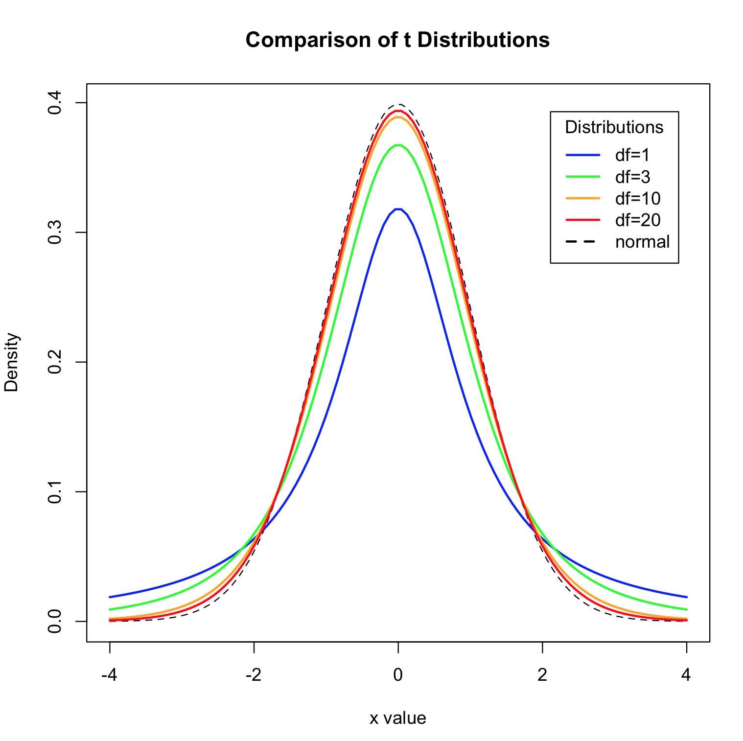
The Student t Probability Distribution
Similar to the normal distribution, the t-distribution is a family of distributions that varies based on the degrees of freedom. A unimodal, continuous distribution, the student’s t distribution has thicker tails than the normal distribution, particularly when the number of degrees of freedom is small. We use the student’s t distribution when comparing means when we do not know the standard deviation of the population and must estimate it from the sample. Above you will find the probability density function of the t-distribution with varying degrees of freedom.