Learning objectives

 

1.  Understand concepts of sample vs. population

2.  Describe data with measures of central tendency

3.  Describe data with measures of dispersion

4.  Understand positive (right) vs. negative (left) skew

5.  Interpret histograms and boxplots

6.  Understand the concept of outliers

 

The following page describes the major concepts and measures in descriptive statistics that may be covered on the statistics diagnostic exam.  I have highlighted the major concepts in green.  Nearly all introductory statistics texts should have a chapter or two on descriptive statistics.

 

Descriptive statistics involves summarizing and organizing the data so they can be easily understood.  Descriptive statistics, unlike inferential statistic, seeks to describe the data, but do not attempt to make inferences from the sample to the whole population.  We typically describe the data in a sample.  A sample is the selected portion of a population, often selected through a random process (such as simple random sampling, or a more complex stratified random sampling approach).  A population is composed of those entities, individuals or objects of interest.  For example, we may be concerned about measuring the diameter of loblolly pines (a coniferous tree common in North Carolina) in a forest tract in the Duke Forest–the population of interest includes loblollys in the forest tract, while the sample would be those trees selected for measurement.

 

 

The data that we collect may be either qualitative (may also be called categorical or nominal) or quantitative (numeric).  Gender, MEM concentration, nation of origin are all qualitative or categorical measures, whereas height, distance, number of students in a class are quantitative.  There is no natural ordering in categorical data, just distinct categories in which an individual/object can be placed.  Quantitative data may either be discrete (such as counts of species occurrence in a plot) or continuous (such as height).

 

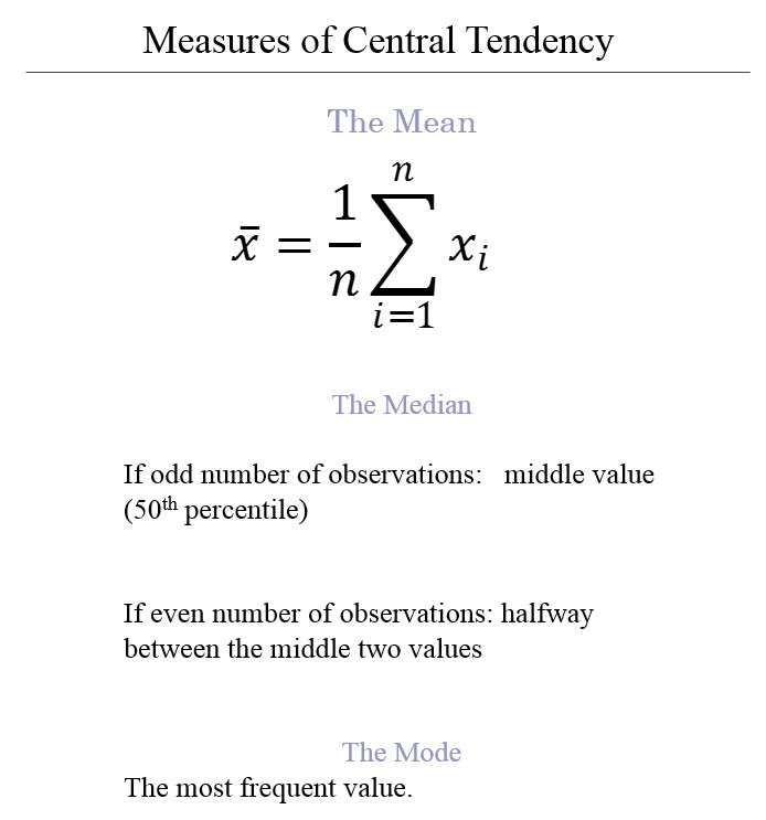
The most basic descriptive statistics include measures of central tendency (mean, median, mode) and measures of dispersion (range, IQR, variance and standard deviation).  We can also discuss the skewness of a distribution.  When a distribution has a right tail it is likely positively skewed.   Alternatively, when a distribution has a left tail, this often suggests a negative (or left) skew.  When the data are normally distributed, the mean, median and mode are equivalent.  However, when the data are right (or positively skewed), the median will be less than the mean.  Alternatively, when the data are left (or negatively skewed), the mean will be less than the median.

 

 

 

 

_________________________

 

Measures of Dispersion

 

_______________________________

 

Histograms

In addition to the basic summary statistics described above, we can also describe the data graphically.  For continuous data, the two most common graphs are the histogram and the boxplot.  The green histogram  below displays the diameter and breast height (DBH) measurements of 250 randomly selected loblolly pines in (imaginary) tract A in the Duke Forest.  The histogram shows no obvious skew, however, the green boxplot below suggests that the distribution of DBH values is positively skewed with four outliers.

 

A Right (Positively) Skewed Distribution

Side-by-Side Boxplots of DBH (cm) of Loblolly Pines in

Tracts A and B

 

Boxplots are another means to display the distribution of data points.  In the boxplots below, one can easily see the median (the solid line in the middle of the box), and the 25th and 75th percentiles (the top/bottom edges of the box).  The IQR is the distance between these edges.  The whiskers extend out from either edge of the box.  In this case (it can vary by software/statistician’s preference), the end of the whisker extends to the point just within the 1.5*IQR + 75th percentile (on the high end) and 25th percentile – IQR*1.5 on the low end of the distribution (these are called the fences).  In this case, outliers are identified as any point outside the fences.  There are four outlier DBH measurements identified in Tract A.  Because of the positive skewness of the data, we would expected the mean to be greater than the median in each of these tracts.  The descriptive (summary) statistics are shown below the boxplots.

 

As we can see in the figure above, four out of the ten distributions contain outliers according to the 1.5*IQR rule, even though the points were randomly drawn from a normal distribution.  This suggests that outliers may occur through a process of random chance.

 

____________________

 

Sample Descriptive Statistics Questions

 

1.  Calculate the mean, median and mode of the following values {2, 4, 4, 4, 12, 12, 20, 110}.

 

2.   True or False:  If a distribution is strongly positively skewed, the median will most likely be greater than the mean.

 

3.   True or False:  If a data set contains an outlier, it should always be eliminated from the data.

 

4.  True or False:  IQR contains 75% of the observations in a distribution.

 

5.    If there is an  outlier in a data set,  its presence most strongly affects which measure of central tendency?

 

 

 SOLUTIONS

Return to the Main Statistics Review home page.

 

This page was developed by Elizabeth A. Albright, PhD of the Nicholas School of the Environment, Duke University.

 

photo credit:  Jeffrey S. Pippen, MS at the Nicholas School of the Environment, Duke University