Skip to content
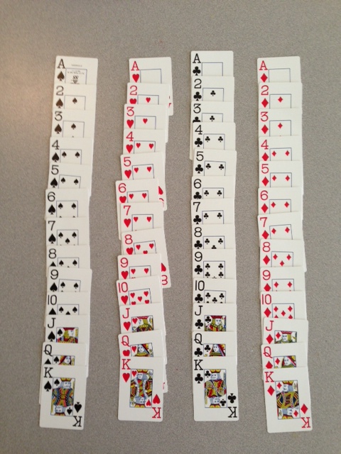
Before we get started on this section, let me introduce to you a deck of cards (inherited from the French several centuries ago). A deck is composed of 52 cards, half red and half black. The red suits are hearts and diamonds while the black are spades and clubs. There are 13 cards in each suit (Ace, 2, 3, 4, 5, 6, 7, 8, 9, 10, Jack, Queen and King). Ace may be either the highest or lowest card (depending on the game).

So now for the probability rules…….
1. A probability may range from zero (0) to one (1), inclusive.
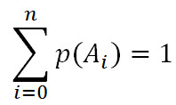
2. The probabilities of all possible outcomes must sum to one. This axiom can be written as:

This is the short hand for writing ‘the sum (the sigma sign) of the probabilities (p) of all events (Ai) from i=0 to i=n equals one’.
3. The probability of an event plus the probability of its complement must equal one.
The addition rule
P(A or B) = P(A) + P(B) – P(A and B)
So back to our deck of cards….We want to know the probability that a drawn card is either a red card (P(A)) OR a seven (P(B)). These two events are NOT mutually exclusive (i.e., a card can be a red AND a seven). So in this case,
P(red or seven) = p(red) + p(seven) – p(red and seven)
P(red or seven) = 26/52 + 4/52 – 2/52 = 28/52 = 7/13
We subtract the 7 of hearts (red) card and the 7 of diamonds card (red) because we don’t want to count these cards twice.
The multiplication rule
(independent events)
If two events are INDEPENDENT (the occurrence of one event does not affect the probability of another event occurring), then
P(A and B) = P(A)P(B)
An example of two INDEPENDENT events are two rolls of a die. The probability of getting a one on the first roll will not affect the probability of getting a one on the second roll. So if we roll the die twice and want to know the probability of getting a one on both rolls:
P(one (roll1) and one (roll2)) = P(one(roll1))*P(one(roll2)) = 1/6 * 1/6 = 1/36
The Law of Large Numbers
The law of large numbers (sometimes named the Law of Averages) states that as the number of trials of a random experiment increases, the empirical probability of an outcome will get closer and closer to its true probability. Or another way of thinking about it, as the number of random trials increases, the expected value of the trial outcomes will approach the true population mean.
So what does this mean? Let’s say we have a fair die, with sides numbered one through six, inclusive. We roll the die six times and count how many times a one appears. The true probability (if the die is fair) of getting a one on each individuals trial is 1/6. However, with our 6 trials, three rolls produced a one (3/6). This is more often than is expected but not totally out of the realm of possibility (we could calculate the probability of this using our probability rules). We know the ‘true’ probability of getting a one on any roll is 1/6. What if we rolled the die 60 times? What’s the likelihood of getting 30 ones?!? Very, very small. We would expect the proportion of rolls coming up one to be closer to 1/6. And with 600 rolls, even closer to 1/6. As the number of trials increases, the long-term frequency, based on our empirical results, will approach the true probability. This is the law of large numbers.
Another way of thinking about the law of LARGE numbers is that the expected value of the observed values will approach the population mean, with increasing number of trials. Here is an external (WH Freeman) link to a Java applet that illustrates the law of LARGE numbers.
Practice Problem
It is estimated that 40% of Durham residents visit Falls Lake in a given year. Three Durham residents are selected at random. What is the likelihood that all three residents visited Falls Lake last year?
Solution
Because the population of Durham is so large (approx. 230,000), we don’t have to worry the issues of replacement vs. non-replacement in our sampling. We can use the multiplication rule above in the form:
P(A and B and C) = P(A)*P(B)*P(C) = 0.4 * 0.4 * 0.4 = 0.064.
Return to the main Probability page.


