Now that we have covered descriptive statistics, probability and sampling, we are ready to make inferences from our sample data to our population of interest.  In statistical inference, we take what we know from the sample, apply the underlying theory of sampling (central limit theorem) to make statements about our population of interest.  We make estimates about the population through the use of the sample data.  Estimates can either be point estimates or interval estimates.   Xbar is an estimator of μ and s (sample standard deviation) is an estimator of σ.   We call the specific value of an estimator the estimate (e.g., 3.5 cm is our estimate of the population mean (μ)).

 

We can also make interval estimates (e.g., we are 95% that the interval (2.0 cm, 5.0 cm) covers the population mean).  And this is where confidence intervals come in!  Remember, every time we sample from a population, the values in the sample are likely to shift because of the random process of sampling.  But to help us, we know that if the sample size is large enough, the MEANS of repeated samples will be normally distributed with a mean of μ and a standard deviation of σ/√n (standard error).

 

So based on the Central Limit Theorem and the three sigma rule, we know that approximately 95% of sample means will be within 2 (1.96 to be more exact) standard errors of the true population mean.  So we could write this out as:

This is our 95% confidence interval.  We can say, with repeated sampling, there is a 95% chance that a random confidence interval will cover the true population mean.  However, it is not correct to say that ONE specific interval (for example (4cm, 12cm) has a 95% probability of covering the true population mean.  We may (and should) say that ‘there is 95% confidence that the interval (4cm, 12cm) covers the true population mean.

Why is our multiplier (z*) 1.96?  Because the area under the standard normal curve between -1.96 and 1.96 is 0.95 (the probability that z is greater than 1.96 is 0.025, as is the probability that z<-1.96.  Together this probability adds to 0.05, or 1 minus the confidence level).  You can calculate a confidence interval with any level of confidence although the most common are 95% (z*=1.96), 90% (z*=1.65) and 99% (z*=2.58).   The generalized confidence interval form, when we know the population standard deviation ( σ) is:

Example Confidence Interval with a Known Population Standard Deviation (σ)

 

For a study we are conducting on nutrition and access to fresh produce in Beaufort County, North Carolina, we want to know how much an adult spends on locally-produced fruit and vegetables in June.  We randomly select 100 individuals from the county property records and send a survey to those residents about their eating, shopping and gardening practices.  With our sample, we find that the average amount an adult spends on locally-grown fruits and vegetables in June is $40.00.  We know from previous studies that the standard deviation of money spent on local produce is $10.  Construct and interpret a 95% confidence interval for the mean (per capita) amount spent on fresh, local produce.

Solution

To construct our confidence interval, we know that the sample mean is $40.00 and the population standard deviation is $10.  Our sample size is 100.  The z* value we will use is 1.96.  Therefore, the confidence interval can be calculated out as:

 

We can conclude that there is 95% confidence that the interval ($38.04, $41.96) includes the true population of money spent on fresh produce by an adult in Beaufort County, North Carolina.

 Interpretation through a Simulation

Using the population distribution we used to demonstrate the CLT, we will now sample (size n = 60) 100 times from this distribution and calculate 100 distinct confidence intervals (95%).  How many confidence intervals would be expect to cover the true population (2.25)?  We would expect about 95% of the intervals to cover (include) the population mean.  As a reminder, here is the population distribution (remember, we typically do NOT know this distribution).

 

 

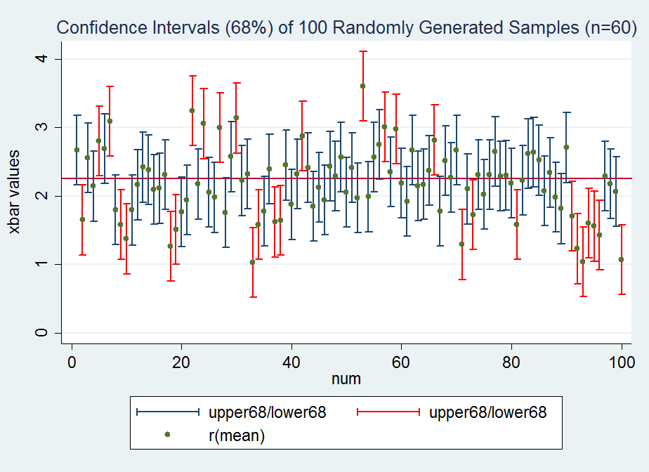
And  here are the confidence intervals of the 100 randomly generated samples (sample size = 60).   Each vertical bar is a confidence interval, centered on a sample mean.  The intervals all have the same length, but are centered on different sample means as a result of random sampling.  The confidence  intervals in red DO NOT cover the true population mean (the horizontal red line μ=2.25).  This is what we would expect using a 95% confidence level.

 

 

Now what would happen if repeat this process, but calculate 68% confidence intervals?  We would expect approximately 68% of the confidence intervals to cover the true population mean.  As you can see the length of each interval has decreased in comparison to the 95% confidence intervals.  Why?  Because we have changed our multiplier (z*) from 1.96 to 1.

 

 

Other scenarios to think about:  What would happen to the length of our confidence intervals if we increase our sample size from 60 to 100?  Would our intervals decrease or increase in length?  What if the population standard deviation increased?

Assumptions behind our Confidence Intervals

 

1.  We assume the standard deviation of the population (σ) is known.

2.  The sample was randomly selected (independence assumption).

3.  The sample size is large enough to insure that the sampling distribution of the sample means is normally distributed.

4.  There are no outliers (extreme high or low values).

 

 

Sample Confidence Interval Problems

 

1. You want to rent an unfurnished one-bedroom apartment in Durham, NC next year.  The mean monthly rent for a random sample of 60 apartments advertised on Craig’s List (a website that lists apartments for rent) is $1000.  Assume a population standard deviation of $400.  Construct a 95% confidence interval.

2. To what population of apartments can you appropriately infer from your sample in #1

3. How large a sample of one-bedroom apartments above would be needed to estimate the population mean within plus or minus $50 with 90% confidence?

4. Duncan Jones kept careful records of the fuel efficiency of his car. After the first 100 times he filled up the tank, he found the mean was 23.4 miles per gallon (mpg) with a population standard deviation of 0.9 mpg. Compute the 95 percent confidence interval for his mpg.

5. Which of the assumptions listed above might be problematic in making inference to the population in Question 4?

6. True or False:  The population mean (μ) is a random variable that will fall within a confidence interval with 95% probability (with repeated sampling).

7. True or False:  With all else constant, an increase in population standard deviation will shorten the length of a confidence interval.